This section discusses typical causal S-Parameters characteristics and displays.  Let us know if you would like the Generate Causal S-Parameters Tool enhanced with additional capability.

A typical SerDes channel, with about 18 nsec time delay, defined for use with serial data at a bit rate of 25 Gbps has its hardware 4-Port S-parameters measured from 10 MHz to 40 GHz in steps of 3.125 MHz as shown here:

Figure 1: S-parameters magnitude response versus frequency; only S21, S41, S23, S24 are displayed

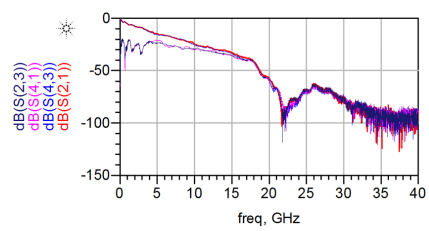
When used as a differential SerDes channel, the ports of this S-parameter data has these assignments:  port 1 is the ‘+’ side input, port 2 is the ‘+’ side output, port 3 is the ‘-‘ side input, and port 4 is the ‘-‘ side output.

As discussed in the article at About Generating Causal S-Parameters, the S-parameters, though measured on actual hardware, actually deviate from the constraints for physical realizability such as passivity, reciprocity, and causality or include noise in the measured S-parameters for various reasons. For physical realizability, the S-parameters should ideally be measured continuously from 0 Hz to infinity and with no noise or distortion. For practical reasons, the S-parameters are band limited, are tabulated only at discrete frequencies, and are corrupted by measurement noise. These measurement limitations typically cause the S-parameters to be non-causal, non-reciprocal, and nonpassive.

The key to obtaining consistent S-Parameter use with any time domain based tool, including any channel simulator, is to convert S-Parameter data to what is called on this web site “Causal S-Parameters”.

The Generate Causal SParameters Tool applies corrections to the original S-parameter data in a proprietary way to meet the constraints for physical realizability and noise reduction. The corrections applied include meeting the mathematical aspects of the Kramers-Kronig relations applied to linear time invariant (LTI) systems.

The causal S-parameters generated will have frequency domain data from 0 Hz to the maximum frequency BitRate*SamplesPerBit/2.  This is the maximum frequency for a discrete time signal defined for use with a sample rate of BitRate*SamplesPerBit. For example, for the band limited S-parameter data discussed above, with BitRate = 25 Gbps and SamplesPerBit = 32, the causal S-parameters will have a maximum frequency of 400 GHz.  The example S-parameter data is band limited to 40 GHz.  The causal S-parameter algorithm used inherently “fills” in the data from 40 GHz to 400 GHz in a causal way without generating any high frequency aliasing.

To generate the causal S-parameters, each Sij value is individually converted to its time domain causal impulse response hij. Thus, for the example 4 port S-parameter data, 16 hij impulse responses are generated. The inverse of this hij data results in the causal Sij data.

The generated causal S-Parameters can be downloaded. The filename will be the concatenation of the original filename + “causal.sp” where = the number of ports for the S-parameter file. The causal S-parameters will extend from frequency 0 Hz to the upper frequency BitRate*SamplesPerBit/2. This means that the original S-parameter data will be extrapolated below its lowest frequency and above its largest frequency as needed.

In addition to the causal S-parameters, the causal impulse responses can be downloaded. The filename will be the concatenation of the S-parameter filename + “.imp”. The causal impulse file has comment lines leading with the “!” character and one format line leading with the “#” character. The format line has the form:

#  Lengths,  <h11_length>,  <h12_length>, …, <hnn_length>
where the <> values are the number of data points for each impulse response.

Thus, a s4p file has 16 impulse lengths in this one format line. The impulse data is in two columns. The first column is for time and the second is the impulse value. The first rows is for the h11 response, the next rows is for the h12 response, etc.

The generated Causal S-Parameters can be compared the original S-parameters.

Let’s look at some of the responses generated for the example S-parameter data.

Figure 2.  S33 (‘-‘ side input) reflection S-parameters.

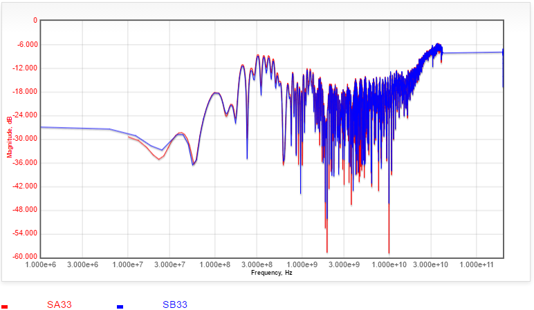
SA33 is for the original data.  SB33 is the causal data.  As can be seen, the causal S-parameters are extrapolated below the original data lower frequency of 10 MHz and above the original data upper frequency of 40 GHz.  In between, the causal S-parameters have close agreement to the original data.

Figure 3.  h33 (‘-‘ side input) time domain impulse response

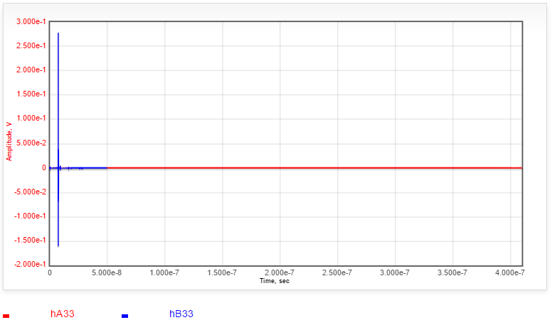
hA33 is for the original data.  hB33 is the causal impulse response.  The data is more revealing when the y axis is on a logarithmic scale as shown here.

Figure 4.  h33 (‘-‘ side input) time domain impulse response with log y axis.

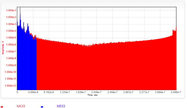
As can be seen, the causal hB33 ends after 50 nsec where as the original data hA33 response is more visibly non causal since its level increases after 180 nsec and has a level that is down only two orders of magnitude at 410 nsec from the level at 8 nsec.

Figure 5.  S21 (‘+’ side input to output) transmission S-parameters.

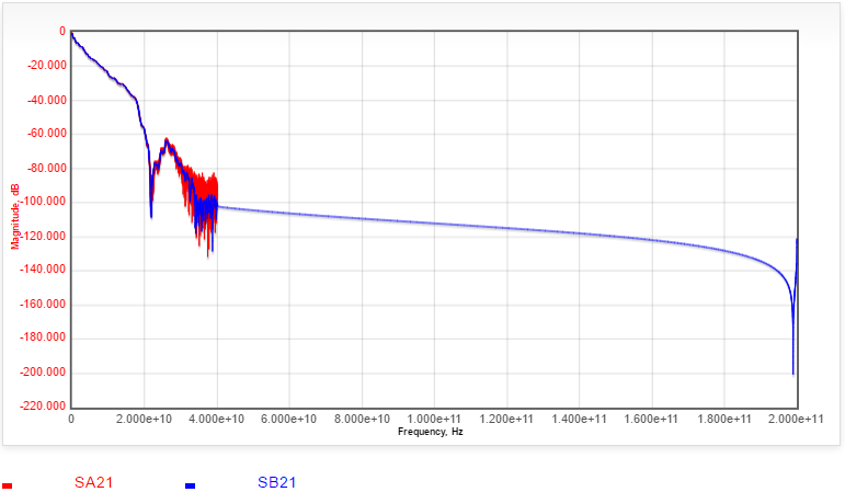
SA21 is for the original data.  SB21 is the causal data.  As can be seen, the causal S-parameters are extrapolated below the original data lower frequency of 10 MHz and above the original data upper frequency of 40 GHz.  In between, the causal S-parameters have close agreement to the original data.  Notice the elimination of the noise above 20 GHz and no high frequency aliasing above 40 GHz.

Figure 6.  h21 (+’ side input to output) time domain impulse response

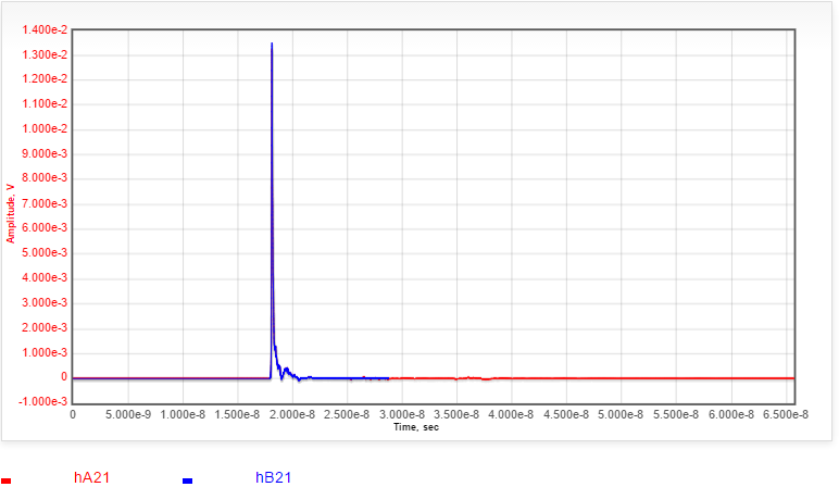
hA21 is for the original data.  hB21 is the causal impulse response.  The data is more revealing when the y axis is on a logarithmic scale as shown here.

Figure 7.  h21 (+’ side input to output) time domain impulse response with log y axis.

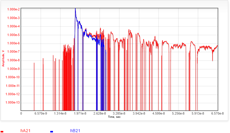
As can be seen, the causal hB21 ends after 30 nsec whereas the original data hA21 response is more visibly non causal and it has a response out to 65 nsec.  Additionally, hB21 has a zero level response for the duration of the channel transmission delay of 18 nsec whereas the original data hA21 has a response before the delay time of 18 nsec which is clearly non-causal.